JERICO – Biofouling Monitoring Program (BMP)
Selected partners and monitoring sites
Partners available to participate actively to the BMP are:
|
N° |
Partners |
Reference person |
|
Coastal Water |
Open Water |
|
1 |
ISMAR |
Marco Faimali |
Please login or register to view contact information.
|
x |
x |
|
2 |
HCMR |
Manolis Ntoumas |
Please login or register to view contact information.
|
x |
x |
|
3 |
AZTI |
Carlos Hernandez |
x |
x |
|
|
4 |
IFREMER |
Laurent Delauney |
x |
x |
|
|
5 |
CEFAS |
Dave Sivyer |
x |
x |
|
|
6 |
SMHI |
Bengt Karlson |
x (?) |
|
|
|
7 |
SYKE |
Jukka Seppala |
x (?) |
|
The following map (figure 1) represents the distribution of 11 different monitoring sites (open water and coastal water) along a European geographical gradient.
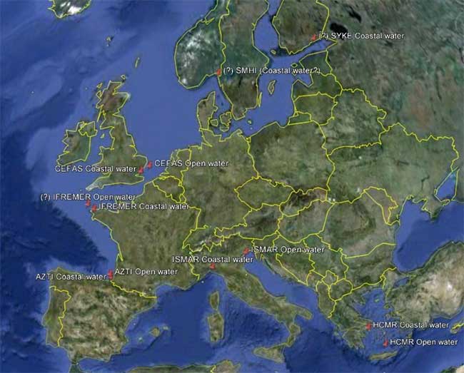
Figure 1: Sampling map
Biofouling Monitoring Box – BMB
ISMAR-CNR developed a special sampling system (Biofouling Monitoring Box – BMB) for each partner and for each sampling site. It will be sent to the address specified by each partner interested in the biofouling monitoring activity.
The BMB is a specifically monitoring device designed to provide substrates with spatial and structural heterogeneity that can simulate the complexity of the sensors and sensor housing/containers.
Each selected partner will immerse the system (BMB) close to a particular sensor, selected as the reference sensor, for this long-term study.
Find below pictures describing the BMB (panels 25×25 cm and tiles 6×6 cm) (Figure 2,3,4):
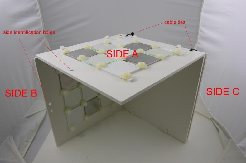
Figure 2: Overview of the biofouling monitoring box (front).
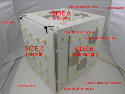
Figure 3: Overview of the biofouling monitoring box (back).
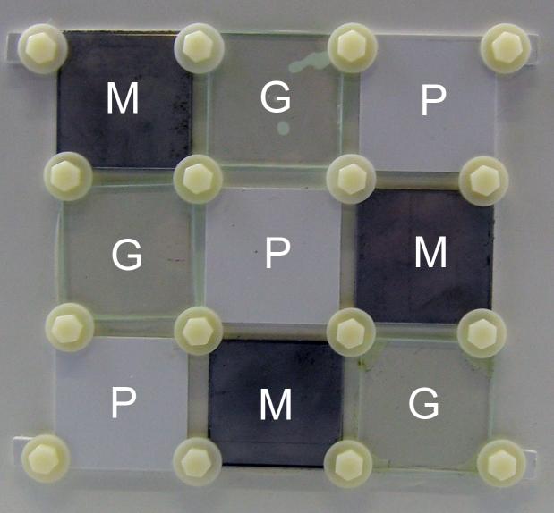
Figure 4: Latin square with 9 tiles of different materials: M= Metal; G=Glass; P=plastic
The BMB is composed of:
– a horizontal side (A), identified by one hole, in which a series of 9 tiles of different materials (Plastic – P; Metal – M; Glass – G) is inserted from both sides (“side up” exposed to light and “side down” exposed to dark).
– a vertical side (B), identified by two holes, with the same series of 9 tiles of different materials on both sides (“side outside” exposed to light and “side inside” exposed to dark)
– a second vertical side (C), with no additional holes, is composed of two panels kept together by cable ties (easily removable to take the photographs). One series of 9 tiles of different materials is inserted between the panels (in order to simulate an interstitial environment in the dark).
On each side bolts will be used as spacers to easily take pictures of all sides avoiding the potential damaging of the corresponding opposite side.
Each partner will photograph the different parts of the BMB and simultaneously the different part of sensor every month, if possible, or at least every 2 months for the coastal monitoring stations and whenever possible to those in the open ocean by following the instructions below. After 6-12 months each partner will ship the two BMBs to ISMAR laboratory after appropriate conservation treatment that is yet to be negotiated.
Protocol for photographic sampling
Once collected the immersed structures from the dive site (BMB and/or reference sensor) run some shots of the complete structure of the BMB and the sensor in order to provide a general overview of them (take pictures from different points of view). A digital camera with a resolution of at least 8MP should be used. The “no flash” option should be selected for all the photos.
BMB
Collect the BMB and bring it to a dry environment waiting for few minutes so that the water can drain off. Place the BMB with the side A (“side up” exposed to light) upwards (as shown in Figure 3). Take a picture of the side A taking into account the holes for sides identification (figure 5 left) and, in macro mode, take a picture for each of the 9 tiles on the side from the top to the bottom and from the left to the right (Figure 7). .
Turn upside down the BMB to photograph the side A exposed to dark , always taking account of the identification holes (figure 5 right). Repeat the same sequence with the panels B (figure 6). Then open the panels of side C cutting the black cable ties and photograph the set of the 9 tiles (figure 8). Replace the two cable ties (figure 9), close the two panels of side C and dip again the BMB in the site. The pictures of the Sides once downloaded on the computer will have to be renamed making clear the Side (A, B, C) and the kind of exposition (light/dark). The pictures of each tile (replicas) have to be renamed considering the material (M, G, P) and replica number (i.e. G1, G2, G3, M1, M2, M3, P1, P2, P3)
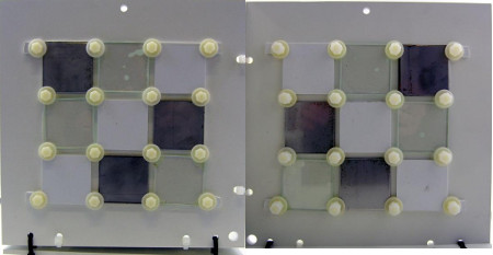
Figure 5: Left: Side A up/light (1 hole on the top, 2 holes on the right), right: side A down/dark (1 hole on the top, 2 holes on the left)
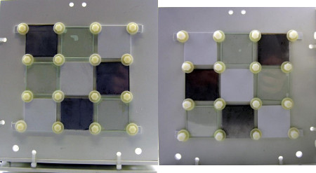
Figure 6: Left: side B outside/light (2 holes on the top, 2 holes on the left); right: side B inside/dark (2 holes on the top, 2 hole on the right)
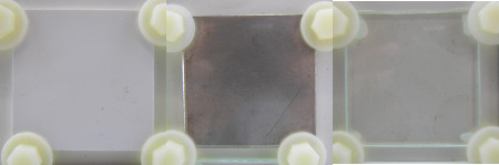
Figure 7: Example of macro pictures of each tile on each side.
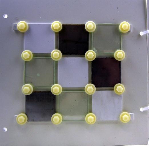
Figure 8: Side C internal
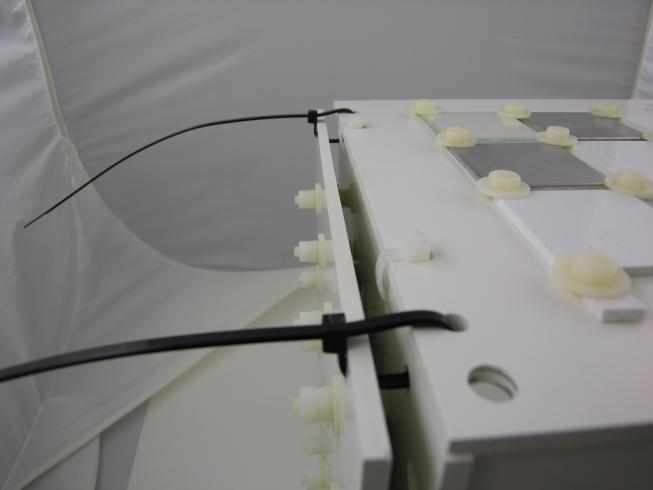
Figure 9: Cable ties to be replaced every photographic sampling session.
Sensors and sensor housing/containers
Depending on the type of sensor selected as the reference for monitoring (BPM) identify the representative areas for sensors and housing / container (different materials, sensitive area). Take pictures in macro mode of the different selected areas so that they are recognizable parts of the sensor to which the macro images relate. One solution might be to assign codes to selected areas (identified by general picture of the structure of the sensor) and name your macro photos with the reference codes.
When you shot sensor parts, remember to place a ruler or a measuring tape to be taken into the picture as size reference.
Overall recommendation for macro shots
Remember each time to photograph the different sides/areas several times (at least 3 repetitions) while maintaining the axis perpendicular to the lens of the camera relative to the surface photographed. This ensures the flatness of the surface to avoid distortions that might affect the subsequent analysis. Macrodigital pictures have to be all consistent in size and light conditions, and close enough to identify the settled organisms. The “no flash” option should be selected for all the photos.
Biofouling estimation
Biofouling coverage will be estimated by Photogrid software (Bird, 2003) and main taxa representative of biofouling community will be recorded in each selected location.
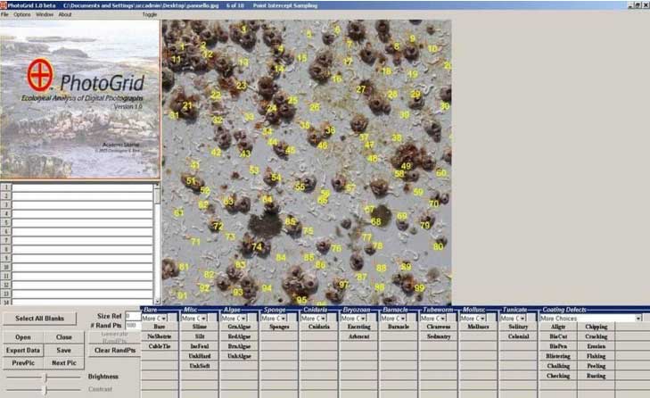
Figure 10: Estimation of biofouling coverage by Photogrid software.
The software creates 100 random points on a digital picture and allows zooming in/out to recognize the main taxonomic groups of biofouling assemblages on a surface (Figure 10). Please note that the ideal condition would be to take the Macro pictures with a quality allowing to obtain cropped images of each tile at least 1000×1000 pixels (the camera quality should be at least 8MP). The output of the software is “total coverage” and percentage coverage for each identified taxonomic group. The main taxonomic groups can be modified and adapted to the local representative species of the considered geographic location.
When the BMB will be collected at the end of the exposure period, the fouled surface will be analysed by standard microscopy techniques and a modified Dethier method (Dethier et al. 1993). The analysis is carried out placing a small grid (20×20 cm) on the sample estimating, in a fixed number of random squares inside the grid, the presence and abundance of each taxa (representative groups of biofouling assemblages) (Figure 11). Each randomly selected square is scored for each identified taxonomic group as follows: 0 absence, 1 if the taxon is covering 1/4 of the square surface, 2 if the taxon is covering 1/2 of the square surface, 3 if the taxon is covering 3/4 of the square surface, 4 if the taxon is covering all the square surface.
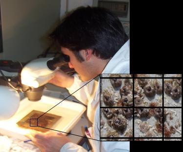
Figure 11: Estimation of fouling by standard microscopy techniques and Dethier method.
Bird C.E. (2003) PhotoGrid version 1.0. Honolulu, Hawaii
Dethier, M. N., E. S. Graham, S. Cohen, and L. M. Tear. (1993). Visual versus random-point percent cover estimations: ‘objective’ is not always better. Mar. Ecol. Progr. Ser. 96: 93-100
Dr. Marco Faimali (PhD)
CNR – Istituto di Scienze Marine (ISMAR) – Sede di Genova
Via De Marini,6 – IV P. – 16149 – GE (I)
Office Phone: +39 010 6475425/428/438
Mobile Phone: +39 347 2772274
Fax: +39 010 6475400
Skype username:balanus66
Web site: http://www.ismar.cnr.it